LLM Speculative Sampling

前言

今天我们将介绍并复现 Deepmind 的一篇关于 LLM Speculative Sampling 的论文：Accelerating large language model decoding with speculative sampling[@sps_deepmind]. 我们将用不到 100 行代码来复现这篇论文，并得到 2 倍以上的速度提升。

比如以当前的 Prompt 为例 (试验采用的 temperature 为 0 以保证确定性)：

Prompt: Alan Turing theorized that computers would one day become

GPT2-XLARGE 的推理的时间为 16.8244 秒：

-------------------- Naive GPT2 Auto-Regressive --------------------
Naive GPT2 Auto-Regressive completed in 16.8244 s
Generated: Alan Turing theorized that computers would one day become so powerful that they would be able to think like humans.

In the 1950s, he proposed a way to build a computer that could think like a human.
(skip ...)
-------------------- Naive GPT2 Auto-Regressive --------------------

推测采样可以生成完全一样的推理结果，且其推理的时间为 7.9031 秒，提升了 2.12 倍：

-------------------- Speculative Sampling --------------------
Speculative Sampling completed in 7.9031 s
Generated: Alan Turing theorized that computers would one day become so powerful that they would be able to think like humans.

In the 1950s, he proposed a way to build a computer that could think like a human.
(skip ...)
-------------------- Speculative Sampling --------------------

简介

Speculative Sampling 中文翻译有多个，这里我们将统一使用推测采样。推测采样是一种大语言模型推理加速的方法。具体来说，推测采样是一种空间换时间的推理加速算法。我们知道，在做一个参数较大的 LLM 模型推理的时候，其推理速度一般会较慢，我们希望能够优化其推理速度。这里我们称待优化的模型为 Target Model。

为了加速其推理速度，推测采样通过引入一个参数量很小的 Draft Model 来一次做多步推理的预测，然后通过一种类似于 Rejection Sampling(拒绝采样) 的方法来保证算法生成的分布和 Target Model 是一致的。推测采样能够生效的关键有两点：Draft Model 的推理速度比 Target Model 要快得多； Draft Model 和 Target Model 具有较高的相似性。在后续的介绍中我们将对这两点进行展开介绍。接下来我们来梳理一下算法的流程。本文中的实验全部基于 GPT2 模型完成，其中 Target Model 为 GPT2-XLARGE，Draft Model 为 GPT2-SMALL。算法实现的全部代码开源在 GitHub: ai-glimpse/toyllm

算法原理

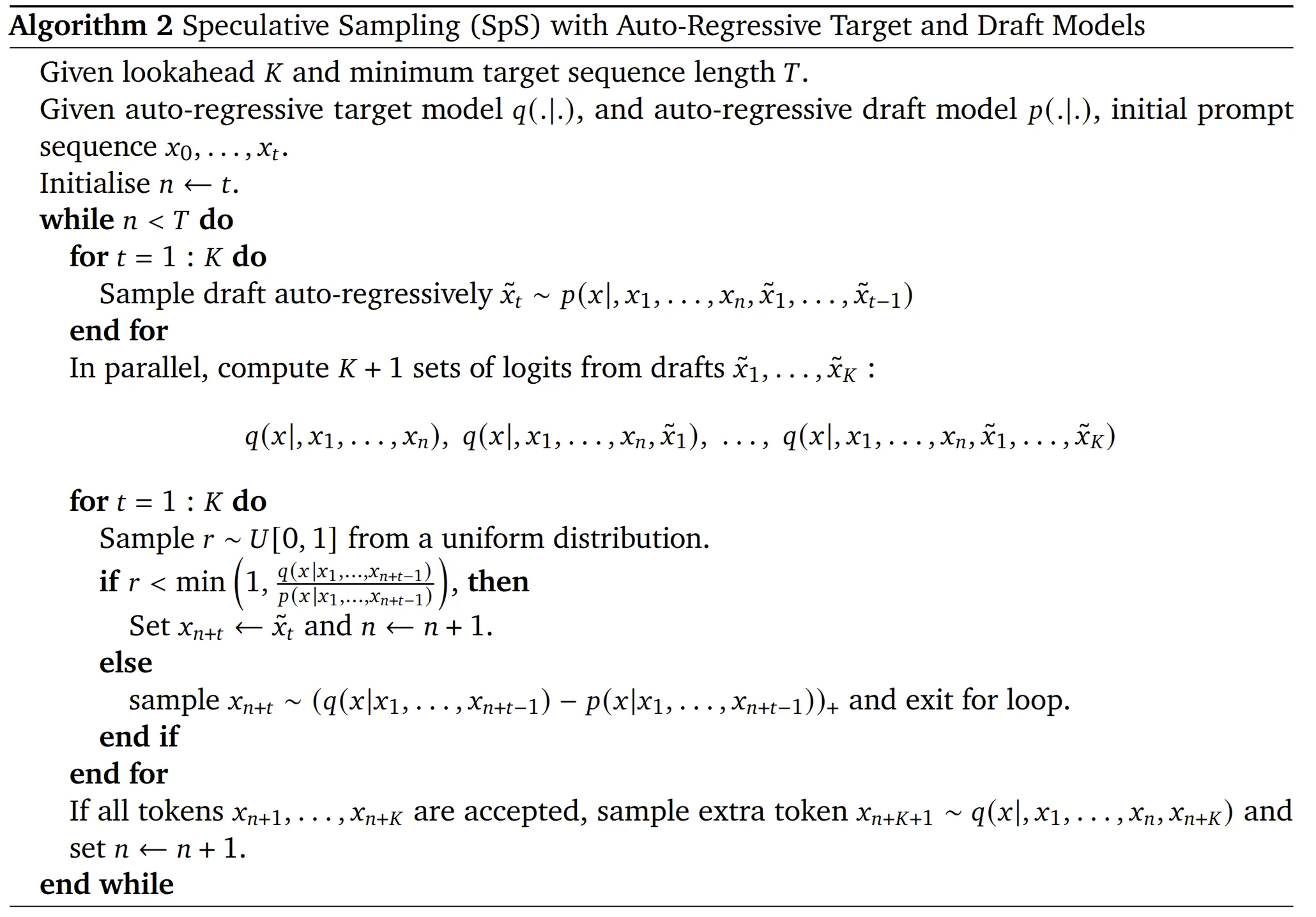
Given lookahead $K$ and minimum target sequence length $T$ .

这里是算法的两个参数 $K$ (lookahead 步长) 和 $T$ (最长生成的 Token 长度). 在之前给出例子中，我们实验用的的 $K=4$ ， $T=266$ .

Given auto-regressive target model $q(\cdot | \cdot)$ , and auto-regressive draft model $p(\cdot | \cdot)$ , initial prompt sequence $x_0,\cdots, x_t$

这里 target model $q$ 就是待优化的参数比较多的模型，比如 GPT-XLARGE，其参数量为 1558M。 draft model $p$ 就是参数较小的模型，比如 GPT-SMALL，其参数量为 124M。 initial prompt 就是一句初始的提示词，比如上面的 Alan Turing theorized that computers would one day become。注意这里 $x_0,\cdots, x_t$ 每个 $x_i$ 代表的是一个 token，而不是一个单词：这里共有 9 个单词，10 个 token. GPT2 模型的 Tokenizer 使用的是 BPE(Byte Pair Encoding), 上述 9 个单词得到的 10 个 Token 如下 (忽略’<>‘符号，主要用于标示出空格)，所以这里的的 $t=9$ 。

1
<Alan>
2
< Turing>
3
< theor>
4
<ized>
5
< that>
6
< computers>
7
< would>
8
< one>
9
< day>
10
< become>

下面是算法运行的主要逻辑：总体流程很简单，就是不断的生成 token 直到生成的 token 长度达到 $T$ 为止。这里有 $t = 9$ , 所以 $n$ 的初始值就是 9； $T=266$ , 所以直到所有 token 的长度达到 266 时算法才会运行结束。具体到代码，也很直观：

1
# Initialise n <- t
2
n = prompt_tokens.size(0)
3
# while n < T do
4
while n < target_seq_len:
5
    ...

接下来进入到 while 循环的内部，首先是第一个 for 循环。

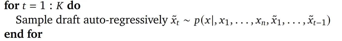
这里的就是对 Draft Model 通过自回归进行采样，共采样 $K$ 个 token.这里的 $K$ 被称为 lookahead 步长，即为前瞻步长，在下面的分析中我们将看到此“前瞻”的具体含义。代码同样也很直观：

1
for _ in range(self.lookahead):
2
    draft_model_probs = self.draft_model.inference(draft_prompt_tokens, config)
3
    next_token_id = torch.multinomial(draft_model_probs[-1], num_samples=1)
4
    draft_prompt_tokens = torch.cat([draft_prompt_tokens, next_token_id], dim=0)

之后是同时计算 target model 的 $K+1$ 份 logits(这里具体是用的归一化之后的 logits，也就是概率，后续我均默认其为概率)。

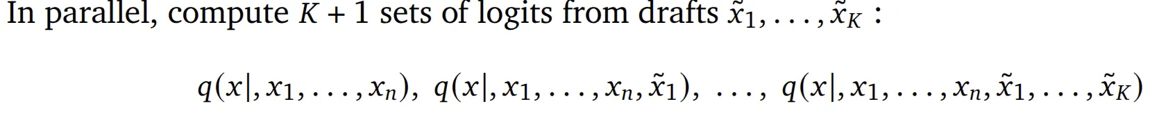
这里其实我们在 target model 进行一次 Forward就可以得到全部的需要的 $K+1$ 份概率分布：

1
target_model_probs = self.target_model.inference(draft_prompt_tokens, config)

接下来就是推测采样的重头戏了。如果说前面的过程是在做出推测，那么接下来的过程就是在验证这个推测的可靠性，并根据可靠与否做出不同的处理。

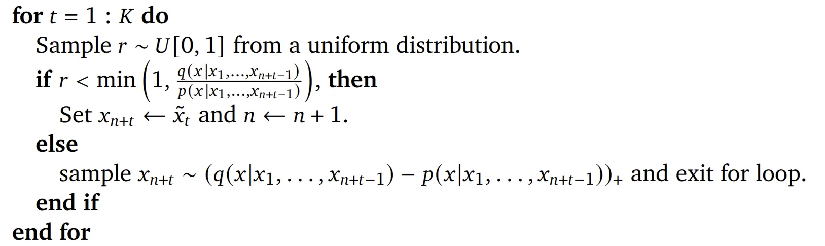
下面的过程是对 draft model 推理出来的 K 个 token 进行逐一验证，我们以第一个 token 为例进行说明，此时 $t=1$ ，那么这里的判断条件就是如下的形式，

r < \min\left(1, \frac{q(x|x_1, \cdots, x_n)}{p(x|x_1, \cdots, x_n)}\right)

其实就是给定当前已经生成的 token，比较 target model 和 draft model 在 token $\tilde{x}_1$ 上的概率值是不是大于 $r$ , 其中 $r \sim U[0, 1]$ ，服从 0 到 1 的均匀分布。如果条件成立，那么就直接采纳当前 token $\tilde{x}_1$ 作为算法的正式输出；否则就拒绝采纳当前 token，并从下面的分布中采样出当前步骤要生成的 token，同时跳出此 for 循环，即结束当前的推测检验过程：

q(x|x_1, \cdots, x_n) - p(x|x_1, \cdots, x_n))_{+}

这里 $(.)_{+}$ 定义如下：

(f(x))_{+} = \frac{\max(0, f(x))}{\sum_{x}{\max(0, f(x))}}

其实就是分布做差，按 0 clip 之后再归一化的过程。

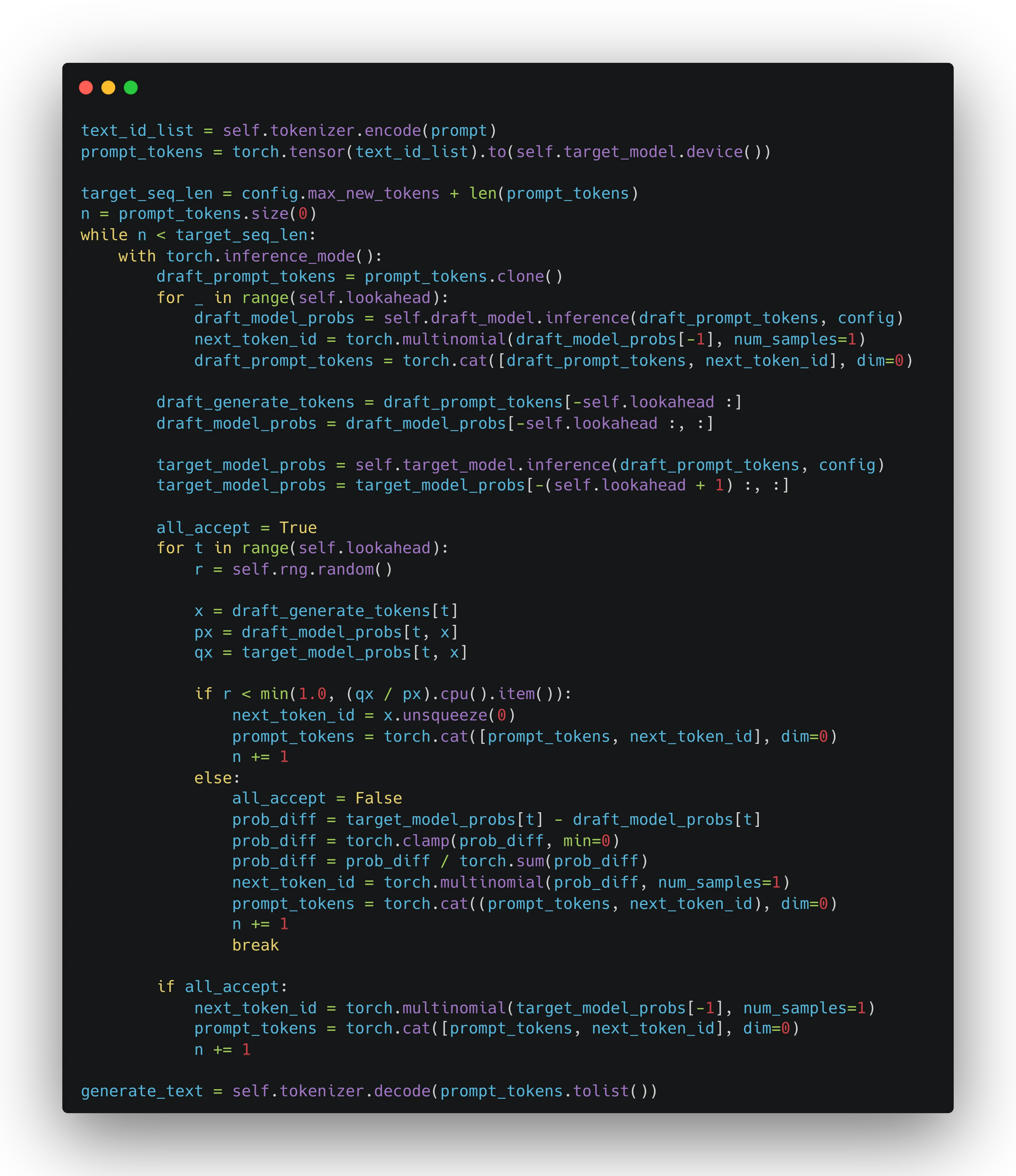
小结一下，在这 $K$ 步检验中，我们对 draft model 生成的 $K$ 个 token 进行逐一检验，如果满足预设的概率条件，那么就采纳此 token 并继续检验下一个推测出来的 token；如果不满足预设的概率条件，重新从“差分布”中采样一个 token 出来，同时结束此轮检验过程。这部分的代码实现如下：

1
all_accept = True
2
for t in range(self.lookahead):
3
    r = self.rng.random()
4

5
    x = draft_generate_tokens[t]
6
    px = draft_model_probs[t, x]
7
    qx = target_model_probs[t, x]
8

9
    if r < min(1.0, (qx / px).cpu().item()):
10
        next_token_id = x.unsqueeze(0)
11
        prompt_tokens = torch.cat([prompt_tokens, next_token_id], dim=0)
12
        n += 1
13
    else:
14
        all_accept = False
15
        prob_diff = target_model_probs[t] - draft_model_probs[t]
16
        prob_diff = torch.clamp(prob_diff, min=0)
17
        prob_diff = prob_diff / torch.sum(prob_diff)
18
        next_token_id = torch.multinomial(prob_diff, num_samples=1)
19
        prompt_tokens = torch.cat((prompt_tokens, next_token_id), dim=0)
20
        n += 1
21
        break

接下来还有 while 循环内最后一小步。

如果 draft model 推测出来的 $K$ 个 token $x_{n+1}, \cdots, x_{n+K}$ 全部被采纳，那么继续从 target model 中采样出下一个 token：

x_{n+K+1} \sim q(x|, x_1, \cdots, x_n, \cdots, x_{n+K})

注意，这里论文中的公式应该是有些小的笔误，下面给出的是修正后的版本。下面是对应的代码实现。

1
if all_accept:
2
    next_token_id = torch.multinomial(target_model_probs[-1], num_samples=1)
3
    prompt_tokens = torch.cat([prompt_tokens, next_token_id], dim=0)
4
    n += 1

至此，算法全部的流程就全部走完一遍了。此时再回顾一下之前的问题——为什么 draft model 生成 $K$ 个 token 的过程叫作 lookahead(前瞻)？答案就比较显然了，其实就是预先推测的意思，这也是推测采样 (Speculative Sampling) 内在的含义。

完整算法代码

在 toyllm项目中可以找到采用此代码实现生成前言中例子的代码。

复杂度分析

在原论文中，其实没有什么复杂度分析的内容，不过 Jay 对复杂度分析的部分做了补充，对于进一步理解推测采样很有帮助。

首先，我们定义以下内容：

$t_{\text{target}}$ : target model 一次推理 (产生一个 token) 需要的时间。论文中的 target model 为 DeepMind 的 70B Chinchilla 模型，推理一个 token 的耗时为 14.1ms
$t_{\text{draft}}$ : draft model 一次推理需要的时间。论文中的 target model 为 DeepMind 的 7B Chinchilla 模型，推理一个 token 的耗时为 1.8ms
$r’$ : Acceptance rate, 接受率。其计算方式为每轮推测采样 (while 循环内) 生成的 token 数量除以 $K+1$ .

因此，不采用推测采样的情况下，target model 进行自回归产生 $N$ 个 token 的时间复杂度为 $N \cdot {t_{\text{target}}}$ .

在采用推测采样的情况下，需要进行多轮循环。每轮循环都涉及到 draft model 的 $K$ 次自回归，和 target model 的 1 次自回归，所以每轮的复杂度为 $t_{\text{draft}}K + t_{\text{target}}$ . 因为接受率为 $r$ ,那么每轮采样出来的 token 数平均就是 $r'(K+1)$ , 那么循环次数就是 $\frac{N}{r'(K+1)}$ . 所以推测采样的复杂度就是如下的形式：

\frac{N}{r'(K + 1)} \cdot (t_{\text{draft}}K + t_{\text{target}})

有了两种方式的时间复杂度，我们就可以算出采样推测采样理论上可以达到的加速倍数：

\begin{align} \text{speedup} & = \frac{\text{time complexity of autoregressive}}{\text{time complexity of speculative}} \\ & = \frac{N\cdot t_{\text{target}}}{\frac{N}{r'(K + 1)} \cdot (t_{\text{draft}}K + t_{\text{target}})} & \\ & = \frac{r'(K + 1) \cdot t_{\text{target}}}{t_{\text{draft}}K + t_{\text{target}}} \end{align}

观察最后的等式，回顾之前提到的推测采样之所以能够加速的两个关键点：draft Model 的推理速度比 target model 要快得多；draft model 和 target model 具有较高的相似性。首先看第一点，draft model 越快，即 $t_{\text{draft}}$ 越小，那么上述公式中的分母就越小，加速比就越大。当其足够小时，我们有如下近似：

\begin{align} \text{speedup} &= \frac{r'(K + 1) \cdot t_{\text{target}}}{t_{\text{draft}}K + t_{\text{target}}} \\ &\approx \frac{r'(K + 1) \cdot t_{\text{target}}}{ t_{\text{target}}} \\ &\approx r'(K + 1) \\ \end{align}

也就是说，加速比与接受率成线性正相关。所以这就引出第二点，即要求 draft model 和 target model 具有较高的相似性。这里的相似性越高， $r'$ 就越高。

下面我们再从试验的角度来分析一下算法的加速比是否符合预期。论文在 HumanEval 和 XSum 分别做了测试 ( $K=4$ )：HumanEval 上的接受率 $r'=0.8$ , XSum 上的接受率为 $r'=0.62$ （来自论文图 1）。对于 HumanEval，代入上面各个参数计算，可以得到其理论上的加速率为 2.65，论文实测得到的加速率为 2.46；同样对于 XSum，其理论上的加速率为 2.05，论文实测得到的加速率为 1.92.

同样地，我们也对前面的例子进行一下复杂度的计算。我们在例子中的 target model 为 GPT-XLARGE(1558M 参数量)，其推理速度为 73.3ms/token，即 $t_{\text{target}} = 73.3$ ；draft model 为 GPT-SMALL(124M 参数量)，其推理速度为 11.9ms/token，即 $t_{\text{draft}} = 73.3$ . 又有平均接受率 $r'=0.8125$ , $K=4$ , 所以我们可以算出在我们的测试中，理论上的加速比例为：

\begin{align} \text{speedup} & = \frac{\text{time complexity of autoregressive}}{\text{time complexity of speculative}} \\ & = \frac{N\cdot t_{\text{target}}}{\frac{N}{r'(K + 1)} \cdot (t_{\text{draft}}K + t_{\text{target}})} & \\ & = \frac{r'(K + 1) \cdot t_{\text{target}}}{t_{\text{draft}}K + t_{\text{target}}} \\ & = \frac{0.8125(4 + 1) \cdot 73.3}{11.9 \cdot 4 +73.3} \\ & \approx 2.46 \end{align}

而我们实测的加速比为 2.12(注意这里我们只是用一个 prompt 做个简单的验算，并没有做严格的 benchmark)，总体还是可以的。

Insight

到这里为止，我们已经把论文中算法的原理梳理清楚，并用代码从头复现了论文，而且最后做了复杂度分析。看起来我们已经完成了复现，但是我在进行到这里的是否总感觉并未“完成”——因为我仍然没有得到对 Speculative Sampling 预期的 insight。或者说，我不觉着自己真正理解了 Speculative Sampling 本身，我知道了算法的 What 和 How，但是对算法为什么真的可以 work 仍然有些说不清的疑惑。所以我试图从别的角度来深入挖掘一下算法本身。

第一个尝试是做数学证明。论文最后给出了当前推测采样得到的分布和 target model 采样得到的分布一致的证明。这个证明很简单，也很容易理解。但是推导完成后对理解算法的本质好像帮助不大。

第二个尝试是深入算法的细节。总览全部算法流程，其实最令人迷惑的地方还是拒绝采样的部分：

r < \min\left(1, \frac{q(x|x_1, \cdots, x_n)}{p(x|x_1, \cdots, x_n)}\right), r \sim U[0, 1]

怎么直观理解这里的采纳条件呢？与此同时，还有另外一个问题，推测采样只保证了分布的相似性，为什么我们之前的测试可以得到完全一致的输出呢？

其实把这两个问题结合起来看，一些 insight 就呼之欲出了。这里的关键在于我们将推理时的 temperature 设置为 0. 当 temperature 为 0 的时候， $q(x|x_1, \cdots, x_n)$ 和 $p(x|x_1, \cdots, x_n)$ 的分布就是词表空间内的离散分布，而且概率密度全部集中在 1 个 token 上，即只有 1 个 token 的概率为 1，其余全为 0. 进一步看，对于 draft model, 因为 $p(x|x_1, \cdots, x_n)$ 就是选中 token 对应的概率密度，所以其在 temperature 为 0 的情况下恒为 1，所以采纳的条件可以简化为下面的形式：

\begin{align} r &< \min\left(1, \frac{q(x|x_1, \cdots, x_n)}{p(x|x_1, \cdots, x_n)}\right) \\ &= \min\left(1, q(x|x_1, \cdots, x_n) \right) \\ &= q(x|x_1, \cdots, x_n) \end{align}

也就是说，这时候采纳的条件退化为 $q(x|x_1, \cdots, x_n)$ 是否大于 $r$ . 因为 $q(x|x_1, \cdots, x_n)$ 也是只在一个 token 上的概率密度为 1，所以这里采纳就只有一种情况，就是 $q(x|x_1, \cdots, x_n)=1$ 的情况，也就是 target model 在 draft model 推测出的这个 token 上的概率也是 1 的情况。简单总结就是，此时已经没有了随机的因素，有的只是对比，对比的是 draft model 和 target model 生成的 token 是否一样。这就是 temperature 为 0 时可以生成完全一样结果的原因。

让我们再深入一些，放开 temperature 为 0 的限制，回归到更加普遍的场景下看这个采纳条件：

r < \min\left(1, \frac{q(x|x_1, \cdots, x_n)}{p(x|x_1, \cdots, x_n)}\right)

可以看到这样的性质：对于 draft model 推测得到的 token $x$ , $q(x|x_1, \cdots, x_n)$ 越大，那么越倾向于采纳此 token；当 $q(x|x_1, \cdots, x_n)$ 很小时，即使 $p(x|x_1, \cdots, x_n)=1$ ，采纳的概率也比较小。

好了，到了这里相信大家对算法的理解又深入了一个层次，我们此次旅程也即将达到终点！最后我来讲一个偶然想到的好玩的问题，供大家讨论娱乐~

我们其实可以调节这里 $r$ 的分布和 $K$ 的大小来达到给模型手动“降智”的目的。比如这里将 $r$ 的分布调节为 $r \sim U[0, 0.5]$ (提高采纳比率), 同时增大 $K$ ,那么就可以提高加速比 (减少了用 target model 推理的次数)：

\text{speedup} \approx r'(K + 1)

其代价就是采样出来的分布不再和 targe model 一致，而是会更加偏向于 draft model，是为“降智”。这种降智来得其实很简单，工程上实现起来也很灵活，比如给某些地区/某些用户都单独配置一个自定义的 $b$ , 使得这些用户推理时 $r \sim U[0, b]$ . 本部分纯属娱乐，大家看着玩就好~

结语

我们本次旅程到此就结束了，祝大家学习愉快！